
Data copied from emails, websites or company systems is often messy: extra spaces, strange hidden characters, and names typed in ALL CAPS or all lowercase. These problems break lookups, create fake duplicates and make reports look unprofessional. Here’s how to clean it fast.
Quick answer: the all-in-one cleaning formula
=PROPER(TRIM(CLEAN(SUBSTITUTE(A2,CHAR(160)," "))))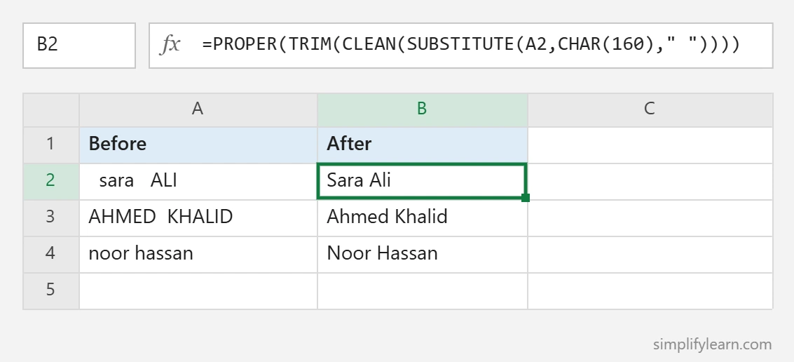
This replaces non-breaking spaces, removes hidden characters, removes extra spaces, and fixes capitalization, all in one step.
Before and after
| Before (A) | After |
|---|---|
| ” sara ALI “ | Sara Ali |
| “AHMED KHALID” | Ahmed Khalid |
| “noor hassan ” (with a hidden line break) | Noor Hassan |
TRIM: remove extra spaces
=TRIM(A2)Removes spaces at the start and end, and reduces multiple spaces between words to one.
Why it matters: “Sara Ali ” (with a trailing space) and “Sara Ali” look identical but aren’t equal. That’s a top cause of #N/A errors in VLOOKUP and XLOOKUP.
CLEAN: remove hidden characters
=CLEAN(A2)Removes non-printing characters (ASCII codes 0–31), such as line breaks and tab marks that come from system exports.
The non-breaking space problem
Data from websites often contains a non-breaking space (character 160). TRIM doesn’t remove it. Replace it with a normal space first:
=TRIM(SUBSTITUTE(A2, CHAR(160), " "))If TRIM “doesn’t work,” this is almost always the reason.
Fix capitalization
| Function | Example result | Use for |
|---|---|---|
=PROPER(A2) |
Sara Ali | Names, cities |
=UPPER(A2) |
SARA ALI | Codes, IDs, country codes |
=LOWER(A2) |
sara ali | Email addresses |
Watch out: PROPER capitalizes after every space and apostrophe, so “McDonald” becomes “Mcdonald” and “o’neil” becomes “O’Neil”. Check special names by hand.
SUBSTITUTE: replace specific characters
- Remove dashes from phone numbers:
=SUBSTITUTE(A2,"-","") - Replace line breaks with a comma:
=SUBSTITUTE(A2,CHAR(10),", ") - Remove all spaces:
=SUBSTITUTE(A2," ","")
Step by step: clean a whole column
- Insert a new column next to the messy data.
- Type the cleaning formula in the first row, e.g.
=PROPER(TRIM(CLEAN(SUBSTITUTE(A2,CHAR(160)," ")))). - Double-click the fill handle to copy it down.
- Copy the new column, then Paste Special → Values (Ctrl + Alt + V → V) over the original.
- Delete the helper column.
Other quick cleaning tools
- Flash Fill (Ctrl + E): type the cleaned version of the first one or two cells, and Excel fills in the pattern for the rest.
- Find & Replace (Ctrl + H): replace double spaces or unwanted text across the sheet.
- Remove duplicates after cleaning. See how to remove duplicates.
- Split names into first and last. See how to split names.
- Power Query: Transform → Format → Trim / Clean / Capitalize Each Word. It’s great for data you clean every month. See Power Query for beginners.
Numbers that won’t calculate?
Spaces and hidden characters can make numbers act like text. After cleaning, wrap the result in VALUE():
=VALUE(TRIM(SUBSTITUTE(A2,CHAR(160),"")))More fixes in numbers stored as text.
Quick summary
- TRIM = extra spaces. CLEAN = hidden characters.
- Use
SUBSTITUTE(A2,CHAR(160)," ")for web data where TRIM doesn’t work. - PROPER / UPPER / LOWER fix capital letters.
- Paste as values when you’re done.