

A normal XLOOKUP finds a value using one condition, like a product ID. But what if you need the price of a product in a specific size, or a sales figure for a specific person in a specific month? Here are three easy ways to use XLOOKUP with multiple criteria.
New to XLOOKUP? Start with XLOOKUP explained.
The example data
| A | B | C | |
|---|---|---|---|
| 1 | Product | Size | Price |
| 2 | T-shirt | Small | 5.500 |
| 3 | T-shirt | Medium | 6.000 |
| 4 | T-shirt | Large | 6.500 |
| 5 | Hoodie | Small | 12.000 |
| 6 | Hoodie | Medium | 13.000 |
| 7 | Hoodie | Large | 14.000 |
Goal: find the price of a Hoodie in size Medium. Put “Hoodie” in F1 and “Medium” in F2.
Method 1: The boolean method (recommended)
=XLOOKUP(1, (A2:A7=F1)*(B2:B7=F2), C2:C7)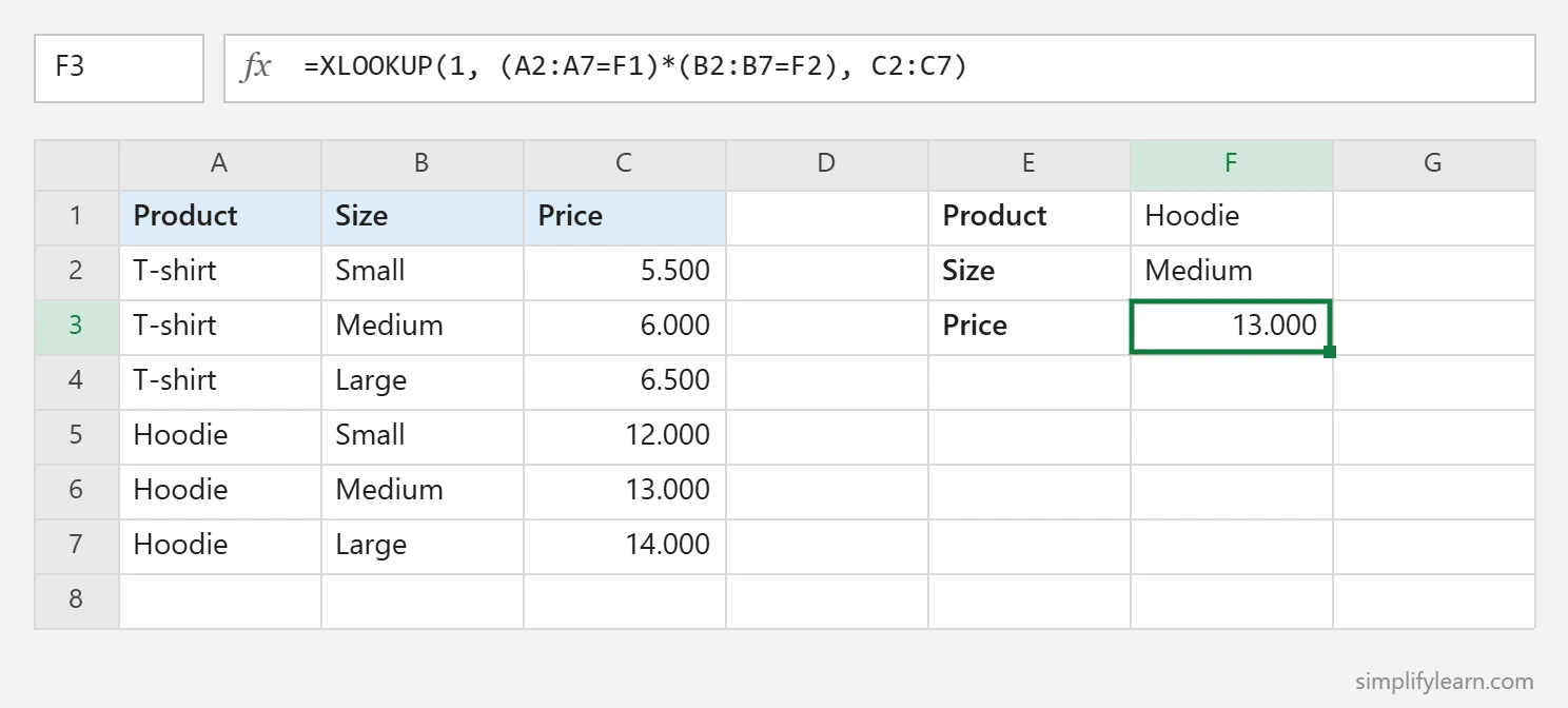
Result: 13.000
How it works:
(A2:A7=F1)checks each row for “Hoodie” → TRUE/FALSE.(B2:B7=F2)checks each row for “Medium” → TRUE/FALSE.- Multiplying them turns TRUE/FALSE into 1/0. A row only gets 1 when both are TRUE.
- XLOOKUP looks for 1 and returns the price from that row.
Add more conditions by multiplying more brackets:
=XLOOKUP(1, (A2:A7=F1)*(B2:B7=F2)*(D2:D7=F3), C2:C7)Use OR instead of AND by adding with + and looking for a value of at least 1:
=XLOOKUP(TRUE, ((A2:A7="Hoodie")+(A2:A7="Jacket"))>0, C2:C7)Method 2: Join the columns
=XLOOKUP(F1&F2, A2:A7&B2:B7, C2:C7)This glues the criteria together (“HoodieMedium”) and searches the glued columns.
Tip: add a separator to avoid accidental matches, for example when “AB”+”C” and “A”+”BC” would both become “ABC”:
=XLOOKUP(F1&"|"&F2, A2:A7&"|"&B2:B7, C2:C7)It’s simple to read, but it only works for exact text matches. Method 1 also handles conditions like “greater than.”
Method 3: FILTER for multiple results
XLOOKUP returns only the first match. To get all matching rows, use FILTER:
=FILTER(C2:C7, (A2:A7="Hoodie")*(C2:C7>12))Result: 13.000 and 14.000. Learn more in UNIQUE, SORT and FILTER.
Add a “not found” message
=XLOOKUP(1, (A2:A7=F1)*(B2:B7=F2), C2:C7, "Not available")Still getting #N/A? Check for extra spaces with TRIM, and see how to fix #N/A.
Criteria with numbers and dates
The boolean method works with any comparison:
=XLOOKUP(1, (B2:B100="Sara")*(A2:A100>=DATE(2026,10,1)), D2:D100)Finds Sara’s first sale on or after 1 October 2026.
Older Excel: INDEX and MATCH
If you don’t have XLOOKUP (Excel 2019 or older):
=INDEX(C2:C7, MATCH(1, (A2:A7=F1)*(B2:B7=F2), 0))In Excel 2019 and earlier, confirm it with Ctrl + Shift + Enter. See INDEX and MATCH explained.
Google Sheets
Methods 1 and 2 work in Google Sheets. Use XLOOKUP the same way. If a formula returns a single value instead of checking every row, wrap it in ARRAYFORMULA().
Quick summary
- Best method:
=XLOOKUP(1, (range1=crit1)*(range2=crit2), return_range). - Simple text matches: join columns with
&. - Need every match? Use FILTER.
- Older Excel: INDEX + MATCH with the same boolean trick.