

Excel’s dynamic array functions changed how spreadsheets work. With one formula you can pull a unique list, sort it, or filter a whole table, and the results update automatically when your data changes. No more copying, pasting and re-sorting.
Works in: Excel for Microsoft 365, Excel 2021, Excel 2024, Excel for the web and Google Sheets (with small differences, explained below).
The example data
A sales table in A1:D9:
| A | B | C | D | |
|---|---|---|---|---|
| 1 | Date | Salesperson | Region | Sales |
| 2 | 01-Oct | Sara | North | 1,200 |
| 3 | 02-Oct | Ali | South | 800 |
| 4 | 03-Oct | Noor | North | 1,500 |
| 5 | 04-Oct | Sara | East | 650 |
| 6 | 05-Oct | Omar | South | 2,100 |
| 7 | 06-Oct | Ali | North | 950 |
| 8 | 07-Oct | Noor | East | 1,750 |
| 9 | 08-Oct | Sara | South | 500 |
What “spilling” means
You type the formula in one cell, and the results “spill” into the cells below and to the right. A blue border shows the spill range. To change the results, edit the first cell. You can’t type inside the spill range.
UNIQUE: get a list without duplicates
=UNIQUE(B2:B9)Result: Sara, Ali, Noor, Omar, one name per row.
Useful options:
=UNIQUE(C2:C9): list of regions=UNIQUE(B2:C9): unique combinations of salesperson and region=UNIQUE(B2:B9,,TRUE): values that appear exactly once
It’s perfect for building a drop-down list that updates itself.
SORT: sort automatically
=SORT(A2:D9, 4, -1)Sorts the whole table by column 4 (Sales), largest first. The arguments are:
- array: what to sort (A2:D9)
- sort_index: which column to sort by (4 = Sales)
- sort_order: 1 = ascending (default), -1 = descending
Combine with UNIQUE for a sorted unique list:
=SORT(UNIQUE(B2:B9))Result: Ali, Noor, Omar, Sara.
SORTBY: sort by another column
=SORTBY(B2:B9, D2:D9, -1)Returns the salesperson names sorted by their sales, highest first, without showing the sales column.
FILTER: show only the rows you want
=FILTER(A2:D9, C2:C9="North")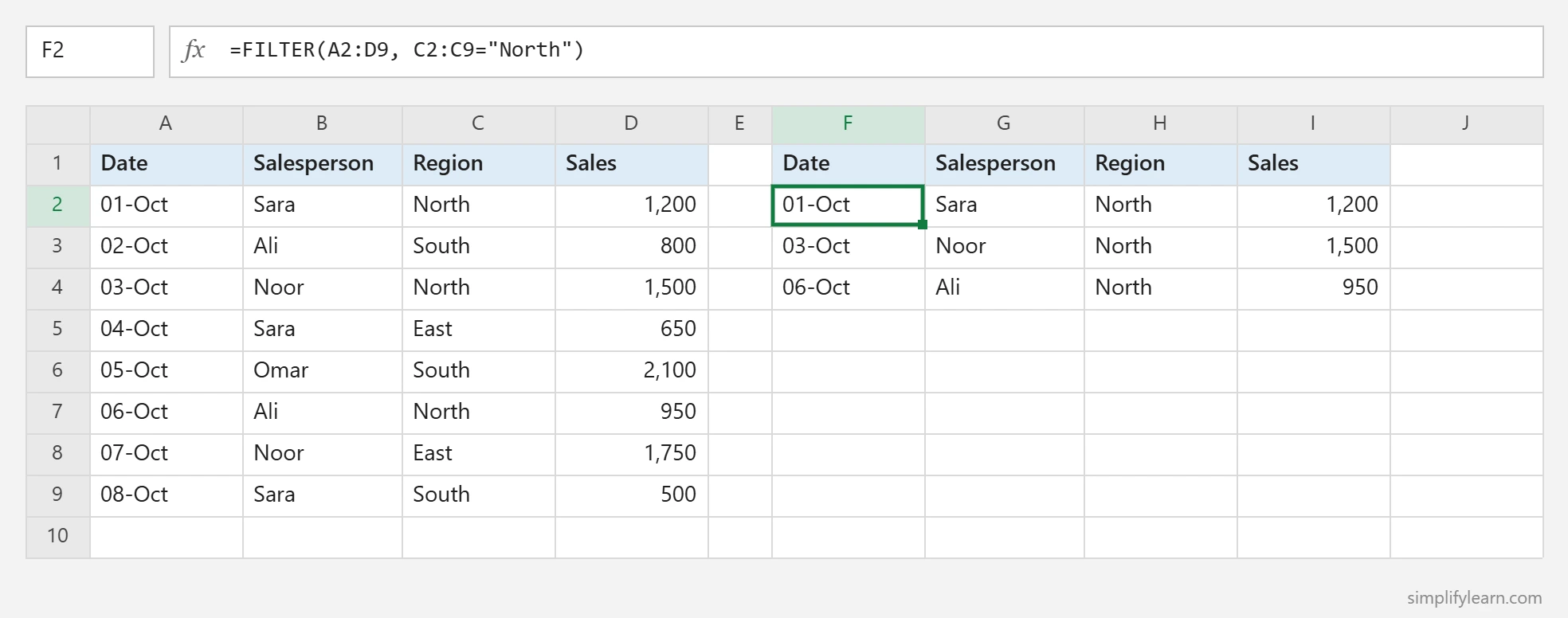
Returns every row where the region is North. The arguments are:
- array: the data to return
- include: the condition (TRUE rows are kept)
- if_empty (optional): what to show if nothing matches
=FILTER(A2:D9, C2:C9="West", "No sales found")FILTER with multiple conditions
AND: multiply the conditions with *
=FILTER(A2:D9, (C2:C9="North")*(D2:D9>1000))North and sales over 1,000 → Sara 1,200 and Noor 1,500.
OR: add the conditions with +
=FILTER(A2:D9, (B2:B9="Sara")+(B2:B9="Ali"))All rows for Sara or Ali.
Use a cell for the condition
Type a region in G1 and use:
=FILTER(A2:D9, C2:C9=G1, "No results")Now you have a mini report that changes when you change G1. Add a drop-down to G1 for a simple dashboard.
Combine them: a top-3 report
=TAKE(SORT(FILTER(A2:D9, C2:C9="North"), 4, -1), 3)Filters North, sorts by Sales (largest first) and keeps the top 3 rows. (TAKE is available in Excel 365 and Excel 2024.)
Fix the #SPILL! error
#SPILL! means something is blocking the results. Usually there’s data in the cells where the formula wants to spill. Click the warning icon to see which cell is in the way, then clear it. Other causes:
- The formula is inside an Excel Table. Dynamic arrays can’t spill inside tables, so put the formula outside the table.
- Merged cells in the spill range.
More on errors in every Excel error explained.
Google Sheets differences
| Function | Google Sheets syntax |
|---|---|
| UNIQUE | Same: =UNIQUE(B2:B9) |
| SORT | =SORT(A2:D9, 4, FALSE) (TRUE = ascending, FALSE = descending) |
| FILTER | =FILTER(A2:D9, C2:C9="North", D2:D9>1000) (each extra condition is ANDed) |
For more powerful reports in Sheets, see the QUERY function.
Quick summary
- UNIQUE removes duplicates from a list.
- SORT / SORTBY sort data automatically.
- FILTER returns only matching rows:
*for AND,+for OR. - Results spill and update automatically. Clear blocking cells to fix #SPILL!.
FAQ
Why do I get #NAME?
Your Excel version doesn’t support dynamic arrays (Excel 2019 or older). Use Sort and Filter buttons or a pivot table instead.
Can I reference the spilled results?
Yes. Add # after the first cell: =COUNTA(F2#) counts everything that F2 spilled.